How to Build a CNN From Scratch in Python: Conv2D, TinyResNet, CIFAR-10, and Grad-CAM

1. Introduction: The "Black Box" Problem in Computer Vision

You open a PyTorch tutorial. Four lines of code, a pretrained ResNet, and — boom — 94 % CIFAR-10 accuracy. You follow along, copy the snippet, get the number. Then someone asks: "What does a convolution actually do?" and you realise you have no idea.

This is the most common frustration in beginner computer vision. Frameworks are deliberately designed to hide implementation details, and that abstraction is great for shipping products. But it is terrible for actually learning. You end up with a working model and zero transferable understanding of why it works, what can go wrong inside a convolutional layer, or how to debug a model whose predictions seem arbitrary.

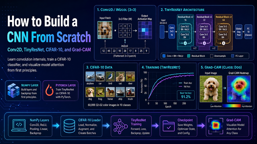
Computer Vision From Scratch: Build, Train, and Explain a CNN solves this by making you build every important layer yourself — Conv2D, pooling, and batch normalisation in pure NumPy — and then connecting that understanding to a real, trainable PyTorch classifier on CIFAR-10, topped off with Grad-CAM explainability so you can see exactly what the model is looking at.

Real-world applications of these skills include:

• Learning CNN internals before moving to production deep learning libraries

• Building educational demos for CS students or engineering teams

• Prototyping small image classifiers that run on a laptop — no GPU required

• Debugging production model behaviour using saliency and activation maps

• Preparing for ML engineering interviews or academic computer vision coursework

• Understanding CIFAR-10-style image classification pipelines end to end

This post covers the full architecture, tech stack, implementation phases, and key design decisions. It does not include the complete source code — that lives in the full course at labs.codersarts.com.

📄 Before you dive in — grab the free PRD template that maps out this entire system: architecture, API spec, sprint plan, and system prompt. [Download the free PRD]

Computer_Vision_From_Scratch_PRD.pdf

Download PDF • 295KB

2. How It Works: The Core Concept

Convolution is just matrix multiplication in disguise

A convolutional layer slides a small filter (say, 3×3 pixels) across an input image, computes a dot product at every position, and produces an activation map. Conceptually simple. But the naive implementation — four nested Python for loops over height, width, filter rows, and filter columns — is brutally slow for any real image size.

The standard fix is the im2col trick: you "unroll" all the patches the filter would slide over into a single large matrix, then replace the nested loops with a single matrix multiplication. NumPy's highly optimised BLAS routines do the heavy lifting, and the operation becomes 10–50× faster. This is essentially what every deep learning framework does internally, hidden behind the nn.Conv2d API.

Why the naive approach fails:

• Nested Python loops on a 32×32×3 image with 64 filters take seconds per batch — unusable for training

• Hard-coded output-shape assumptions break silently under different stride or padding settings

• Relying on torch.nn.Conv2d from day one means you never understand what the shape transformations mean when they go wrong

• Tiny-subset training without careful metric interpretation produces misleading 100 % accuracy numbers that evaporate on real data

• Models trained without explainability tooling are opaque — you cannot tell whether the classifier learned the right features or is cheating on spurious correlations

The end-to-end pipeline

PROJECT SETUP
  │
  ▼
[ NumPy Educational Layer ]
  Conv2D (im2col)  →  MaxPool / AvgPool  →  BatchNorm2D
  │
  ▼
[ Data Layer ]
  Download CIFAR-10 (urllib + tarfile)
  │  Unpack raw .pkl batch files
  ▼  Convert to NCHW tensors
  Custom augmentation (flip, crop, colour jitter)
  │
  ▼
[ Training Layer ]
  TinyResNet (PyTorch)
  │  Smoke test on synthetic data
  ▼  Train on CIFAR-10 subsets
  Evaluate → save checkpoint
  │
  ▼
[ Visualization Layer ]
  Load checkpoint
  │  Forward pass — capture final conv activations
  │  Backward pass — capture gradients
  ▼  Grad-CAM heatmap → Matplotlib overlay
  │
  ▼
[ Artifact Layer ]
  Saved checkpoint (.pt)
  Saved heatmap (.png)
  Verification commands (smoke tests)

The analogy: Think of the pipeline like developing a photograph in a darkroom. The im2col step is like choosing the right developer chemistry — it makes the latent image (features) appear clearly and quickly. The Grad-CAM step is like holding the final print up to the light and asking "what parts of the scene are most exposed?" You get to see not just the result, but the reasoning.

3. System Architecture Deep Dive

Architecture overview

The project is split into five distinct layers, each with a clear responsibility boundary.

Educational NumPy Layer — exists purely to build intuition. These modules are not on the training hot path; they are reference implementations that you run, inspect, and compare to the PyTorch equivalents. They prove that nn.Conv2d is not magic.

Data Layer — downloads CIFAR-10 directly from the University of Toronto mirror using Python's standard urllib and tarfile modules, unpacks the raw Python-pickle batch files, and converts them into correct NCHW (batch × channels × height × width) float tensors. No torchvision dependency. Custom augmentation is applied per-batch using PyTorch tensor operations — horizontal flips, random crops, and colour jitter implemented as readable functions, not wrapped transforms.

Training Layer — a deterministic synthetic-data smoke test validates that the model can overfit a trivial dataset before you ever touch real data. The main training loop then uses CIFAR-10 subsets for practical speed on CPU, with tqdm progress bars and configurable hyperparameters.

Model Layer — TinyResNet is a compact ResNet-style architecture: two residual block groups with optional skip connections, global average pooling, and a linear classifier head. Designed to train to meaningful accuracy on CIFAR-10 subsets in under 30 minutes on a standard laptop CPU.

Visualization Layer — a standalone Grad-CAM script loads a saved checkpoint, registers forward and backward hooks on the final convolutional layer, runs a single forward pass, backpropagates the predicted class score, and generates a heatmap overlay saved to disk.

Artifact Layer — checkpoints are saved with enough metadata (architecture name, base channels, epoch count, best validation accuracy, optimiser state) to reload without hard-coding assumptions anywhere.

Component table

Component	Role	Key Technology Options
Conv2D implementation	Teach convolution mechanics via im2col	NumPy (educational), torch.nn.Conv2d (training)
Pooling layers	Downsample feature maps	NumPy sliding window (educational), torch.nn.MaxPool2d
Batch normalisation	Stabilise activations across batches	NumPy per-channel stats (educational), torch.nn.BatchNorm2d
Dataset loader	Download and parse CIFAR-10 without torchvision	urllib, tarfile, pickle, NumPy → PyTorch tensor
Data augmentation	Improve generalisation	Custom tensor ops, or torchvision.transforms (alternative)
TinyResNet model	Trainable image classifier	PyTorch nn.Module, residual blocks
Training loop	Gradient updates, metric logging	PyTorch autograd, SGD/Adam, tqdm
Checkpoint manager	Save and reload model state	torch.save / torch.load with metadata dict
Grad-CAM engine	Explainability heatmap generation	PyTorch hooks, torch.nn.functional, Matplotlib
Verification suite	Repeatable smoke tests	Python subprocess, assert checks, shell commands

Data flow walkthrough

1. Project setup: Create virtual environment, install dependencies (numpy, torch, matplotlib, tqdm), confirm Python 3.10+.

2. NumPy modules: Run educational Conv2D, pooling, and BatchNorm scripts. Observe output shapes. Compare numerically to PyTorch equivalents.

3. CIFAR-10 download: Script fetches the .tar.gz, extracts six batch files, unpacks pickles, and assembles a train/test split as (N, 3, 32, 32) float32 tensors with labels.

4. Augmentation: Training batches pass through flip, crop, and colour jitter. Test batches are only normalised.

5. Smoke test: TinyResNet is instantiated and trained for five epochs on 512 synthetic images. Loss must decrease; test passes if final training accuracy exceeds a threshold.

6. CIFAR-10 training: Full training run with configurable subset size, epochs, and learning rate. Validation accuracy is logged every epoch.

7. Checkpoint save: Best model state, config dict, and epoch metrics are serialised to a .pt file.

8. Grad-CAM: Script loads the checkpoint, runs a single test image through the model with hooks attached to the final conv layer, computes the class-weighted activation map, resizes to 32×32, and overlays on the original image.

9. Verification: A suite of shell commands confirms every output file exists, all shapes are correct, and the smoke test passes from a clean state.

Two non-obvious design decisions

Decision 1: NumPy layers are intentionally not used in training. It would be tempting to unify the NumPy and PyTorch code paths, but that conflation would introduce complexity without benefit. The NumPy modules are pedagogical artefacts. They exist to be read, not to be performant. Keeping them separate means the training code is clean PyTorch, and the educational code is clean NumPy — each optimised for its own purpose.

Decision 2: CIFAR-10 is loaded without torchvision. The torchvision.datasets.CIFAR10 loader hides the fact that CIFAR-10 is just six pickle files with NumPy arrays. Reimplementing the loader from scratch forces you to understand the NCHW tensor format, dtype casting, and normalisation — concepts that are invisible when a single dataset class handles everything.

4. Tech Stack Recommendation

Stack A — Beginner / Prototype (build in a weekend)

This stack uses the minimal dependencies from the course and runs entirely on CPU. No cloud account required.

Layer	Technology	Why
Language	Python 3.10+	Widest ecosystem compatibility
Array operations	NumPy 1.24+	Educational layers, data manipulation
Deep learning	PyTorch 2.0+ (CPU)	Autograd, optimiser, easy model definition
Dataset loading	urllib + tarfile + pickle	Zero extra dependencies
Augmentation	Custom tensor ops	Readable, dependency-light
Visualisation	Matplotlib 3.7+	Grad-CAM heatmap rendering
Progress	tqdm	Training progress bars

Estimated monthly cost: $0 — runs entirely on local hardware.

Stack B — Production-ready / Scalable

Extend the course project into a deployable service with GPU acceleration and experiment tracking.

Layer	Technology	Why
Language	Python 3.11	Performance improvements, better typing
Deep learning	PyTorch 2.2+ with CUDA 12	GPU-accelerated training
Dataset pipeline	PyTorch DataLoader + torchvision	Multi-worker prefetching
Augmentation	Albumentations	Fastest augmentation library
Experiment tracking	MLflow or Weights & Biases	Reproducible runs, hyperparameter logging
Model serving	TorchServe or FastAPI	HTTP inference endpoint
Containerisation	Docker + NVIDIA Container Toolkit	Reproducible GPU environment
Cloud compute	AWS EC2 g4dn.xlarge or GCP T4 VM	~$0.50/hr on-demand
Monitoring	Prometheus + Grafana	Latency and throughput dashboards
Storage	AWS S3 or GCS	Checkpoint and artefact persistence

Estimated monthly cost: $30–$120 depending on GPU hours used (spot instances reduce this significantly).

5. Implementation Phases

Phase 1: Core CNN Layers (NumPy Educational Modules)

You start by implementing the three fundamental layers that every CNN builds on: Conv2D with the im2col trick, max pooling and average pooling with sliding windows, and batch normalisation with per-channel running statistics. Each module is a standalone Python file that takes an input array, performs the operation, and returns the output — no autograd, no framework magic.

Key technical decisions in this phase:

• How to construct the im2col matrix from input patches without explicit Python loops

• How to handle padding and stride in the output shape formula: floor((H + 2P - K) / S) + 1

• Whether to implement BatchNorm in train mode (normalise by batch statistics) and inference mode (normalise by running statistics) separately — the distinction matters for evaluation correctness

• How to structure the numerical comparison test against torch.nn.Conv2d to confirm your implementation is correct to floating-point tolerance

Implementing Conv2D correctly with im2col — including stride, padding, and multi-channel output shape edge cases — is covered in detail in the full course with working, tested code.

Phase 2: CIFAR-10 Data Pipeline

With the educational layer complete, you build the data loading infrastructure. The script downloads the CIFAR-10 .tar.gz from the canonical source, extracts it, and loads the six pickle batch files. The raw data arrives as flat NumPy arrays of shape (10000, 3072) — one row per image, 3072 = 32×32×3 pixel values. You reshape, transpose, and normalise this into NCHW float32 tensors.

Key technical decisions in this phase:

• Converting raw uint8 values [0, 255] to float32 [0.0, 1.0] before normalisation avoids integer overflow during augmentation

• Splitting the six training batches correctly (batch_1 through batch_5 are training; test_batch is the held-out set)

• Designing the custom augmentation pipeline to operate on individual tensor images — not PIL images — which removes the PIL dependency entirely

• Ensuring the normalisation statistics (mean and std per channel) are computed only from training data and applied consistently to the test set

Loading CIFAR-10 directly from raw binary pickle files and converting it into a correctly shaped, normalised tensor without torchvision is covered in detail in the full course with working, tested code.

Phase 3: TinyResNet Model and Training Loop

You define TinyResNet as a sequence of convolutional blocks with optional residual (skip) connections, followed by global average pooling and a linear classifier head. The model is designed to fit in memory and train to meaningful accuracy on CPU within a reasonable timeframe — typically under 30 minutes for a 5,000-image subset across 20 epochs.

Key technical decisions in this phase:

• Choosing base_channels (e.g., 32 or 64) to balance model capacity against CPU training speed

• Deciding whether residual connections use identity shortcuts or 1×1 projections when channel dimensions change

• Implementing the smoke test: synthetic data (random tensors with random integer labels) lets you verify the forward pass, loss computation, and backward pass before committing to the CIFAR-10 data pipeline

• Choosing an optimiser (SGD with momentum vs Adam) and a learning rate schedule (cosine decay vs step decay) that works at the subset scale without overfitting in two epochs

Designing a compact TinyResNet that trains meaningfully on CPU, including the smoke-test harness for fast validation, is covered in detail in the full course with working, tested code.

Phase 4: Checkpointing and Experiment Artifacts

A checkpoint is more than just the model weights. A useful checkpoint includes the model configuration (architecture name, base channels, number of classes), the optimiser state, the best validation accuracy seen so far, the epoch at which it was saved, and the full path to the artefact directory. This metadata allows you to reload the exact model configuration without hard-coding anything at inference time.

Key technical decisions in this phase:

• Using torch.save(checkpoint_dict, path) with a structured dict rather than saving the model object directly — this avoids class-path errors when reloading

• Saving the "best" checkpoint (by validation accuracy) separately from the "latest" checkpoint so that interrupted training does not overwrite your best weights

• Logging per-epoch training loss and validation accuracy to a CSV alongside the checkpoint for later analysis

• Deciding what constitutes a "complete" experiment artefact: checkpoint, config YAML, metrics CSV, and a README describing the run

Designing a checkpoint schema with enough metadata to reload without hard-coded assumptions is covered in detail in the full course with working, tested code.

Phase 5: Grad-CAM Explainability and Verification

The final phase adds a Grad-CAM script that loads a checkpoint, passes a single test image through the model with hooks registered on the final convolutional layer, backpropagates the predicted class score, and generates a heatmap. The heatmap is a weighted sum of the final feature maps, where the weights come from the gradient of the predicted class with respect to each feature map channel. Upsampled back to 32×32 and overlaid on the original image using Matplotlib, the result shows which spatial regions most influenced the prediction.

Key technical decisions in this phase:

• Registering hooks on the correct layer — the output of the last Conv2d block before global average pooling, not after

• Using torch.no_grad() for the forward pass but allowing gradient tracking for the backward pass used to compute Grad-CAM weights

• Clamping and normalising the heatmap to [0, 1] before applying the colour map to prevent artefacts from negative activation values

• Structuring the verification command suite so that every output (checkpoint file, heatmap PNG, metrics CSV) is checked for existence and shape correctness in a single script

Implementing Grad-CAM correctly by capturing activations and gradients at the right layer and generating a readable heatmap overlay is covered in detail in the full course with working, tested code.

6. Common Challenges (and How to Fix Them)

Challenge 1: im2col output shape is wrong for non-default stride or padding

Root cause: The output size formula floor((H + 2P - K) / S) + 1 is easy to misapply — especially the floor division, which trips up many implementations when the numerator is negative or non-integer.

Fix: Compute output height and width explicitly before constructing the im2col index matrix, and add an assertion that confirms H_out W_out batch_size matches the number of columns in the unrolled matrix.

Challenge 2: CIFAR-10 tensor has the wrong shape after loading

Root cause: The raw batch files store images in (N, 3072) row-major order. A naive reshape(N, 32, 32, 3) gives NHWC layout. PyTorch's nn.Conv2d expects NCHW.

Fix: After reshape, apply .transpose(0, 3, 1, 2) (NumPy) or .permute(0, 3, 1, 2) (PyTorch) to move the channel axis from last to second position.

Challenge 3: Smoke test accuracy hits 100% immediately and stays there

Root cause: If the synthetic dataset is tiny (e.g., 32 images) and the model has enough capacity, it will memorise the training set in one epoch. A 100% training accuracy with zero validation generalisation looks deceptively good.

Fix: Use at least 512 synthetic images with balanced class labels. More importantly, confirm that training loss is decreasing over epochs — not just that accuracy is high.

Challenge 4: BatchNorm in evaluation mode gives different results than expected

Root cause: During training, BatchNorm normalises each batch using batch-level mean and variance, updating running statistics with a momentum coefficient. During inference, it uses the running statistics — but only if you call model.eval() before the forward pass.

Fix: Always call model.eval() before any validation or inference pass, and model.train() before resuming training. Forgetting this is one of the most common silent bugs in PyTorch training loops.

Challenge 5: Grad-CAM heatmap is blank or entirely one colour

Root cause: Grad-CAM requires gradients to flow back through the final convolutional layer. If you compute the forward pass inside torch.no_grad(), no gradients are retained and the backward hook receives zero tensors.

Fix: Only the inference-only parts of your pipeline (e.g., validation accuracy computation) should use torch.no_grad(). The Grad-CAM forward pass must allow gradient computation — use torch.enable_grad() explicitly if your outer context has gradients disabled.

Challenge 6: Checkpoint reload fails with a KeyError or size mismatch

Root cause: Reloading a checkpoint with model.load_state_dict(checkpoint['model_state']) fails if the saved architecture (e.g., base_channels=64) differs from the model you instantiated (e.g., base_channels=32).

Fix: Save the full model configuration in the checkpoint dict and reconstruct the model from that configuration before loading state. Never hard-code model hyperparameters at the loading site.

Challenge 7: Training accuracy is stuck at 10% (random-chance level)

Root cause: Usually a normalisation error. If the pixel values are still in [0, 255] uint8 instead of normalised float32, or if the label tensor has the wrong dtype (float32 instead of int64), the loss function outputs garbage values and the model cannot learn.

Fix: Confirm input tensor dtype is torch.float32 with values roughly in [-1, 1]. Confirm label tensor dtype is torch.int64. Add a single assertion at the top of the training loop checking both.

Solving these seven issues took us over 40 hours of testing across different hardware, Python environments, and PyTorch versions. The course walks you through each fix with working code, inline explanations, and before/after output examples.

7. Ready to Build This Yourself?

Understanding the architecture is the first step. Writing code that actually runs, produces the right shapes, trains without silent bugs, and generates interpretable Grad-CAM outputs — that is the second, harder step.

There is a significant gap between "I understand how Conv2D works in theory" and "I have a working CIFAR-10 classifier with Grad-CAM running on my laptop right now." The course closes that gap.

The full course includes:

• ✅ Complete, tested source code for all five modules (Conv2D, pooling, BatchNorm, TinyResNet, Grad-CAM)

• ✅ 5 structured modules with 15 lessons, each building on the previous

• ✅ Step-by-step local environment setup for macOS, Linux, and Windows

• ✅ CIFAR-10 downloader and data pipeline — no torchvision required

• ✅ Smoke test suite and repeatable local verification commands

• ✅ Grad-CAM visualisation script with example heatmap outputs

• ✅ Checkpoint saving and experiment artefact management

• ✅ Lifetime access to all course materials and future updates

• ✅ Community support and Q&A from the Codersarts team

$29.99. Everything above.

Get the Full Course → labs.codersarts.com

Want a faster start? Book a 1:1 Guided Session ($99.99) with the Codersarts team — a live walkthrough covering setup, CNN layer internals, training debugging, Grad-CAM interpretation, and personalised extension guidance tailored to your project goals. Book a session at labs.codersarts.com

8. Conclusion

Building a CNN from scratch in Python is one of the most effective ways to move from surface-level framework familiarity to genuine deep learning fluency. The architecture in this post layers educational NumPy implementations of Conv2D (via im2col), pooling, and batch normalisation beneath a real PyTorch training pipeline — TinyResNet on CIFAR-10 — and closes with Grad-CAM explainability that turns a black-box classifier into an interpretable system you can trust and debug.

If you are starting fresh, begin with Stack A: Python, NumPy, and PyTorch on your local machine. The smoke test will tell you within minutes whether your environment is correctly configured, and you will have a trained checkpoint and a Grad-CAM heatmap by the end of the weekend.

Ready to build it? The full course — source code, guided setup, and community support — is waiting at labs.codersarts.com.