Tableau Charts (Part IV): Fill maps, Histograms and Boxplots.
- Jul 13, 2021
- 5 min read
Updated: Jun 1, 2023

This is the fourth blog in the Tableau charts series where we explore different charts offered in Tableau. In the previous blog we discussed pie charts, doughnut charts and scatterplots in detail, today, we will learn how to make Fill maps, Histograms, Boxplots and Word cloud.
So get your reading glasses on (only if you need any :) ).
You can check out the previous blog here.
If you are following this series of blog then you know the drill. But for the new comers I will repeat it:
We will be using the Superstore dataset. Although it is already available in Tableau please download it from below here since some changes have been made to it for the purpose of this tutorial.
Just load the data and get to the workspace so that we can begin. In case you don't know how to please refer to this blog.
Fill maps
Fill map is a chart type in which different geographic territories can be represented on the map with areas colored based on a measure or dimension.
Fill maps are a concise way to visualize a large geographical data. You can also use a Bar chart to display a similar data but if the data is too large, reading a bar chart would become a hassle.
To make a fill map you can drag a geographical field onto the 'Details' option on the marks card and Tableau would automatically build a fill map for you. For e.g. drag the field 'Country/Region' to the 'Details' option. It's that easy.
But of course, there are alternative ways to do the same.
You can either drag the 'latitude' and 'longitude' to the rows and columns shelves respectively and then drag the 'Country/Region' to the 'Details' option on marks card or you can use the 'Show Me' option as well. For that you can drag a geographical data (Country/Region, State, etc.) to one of the shelves and then select the maps option from the 'Show Me' Tab.
To add more details you can drag the desired fields to the required options on the marks card. Let us make our fill map a bit more detailed. As of now our fill map is just showing the country/region which is just 'United State'. This doesn't provide us with any meaning full analysis. Let's bring in the 'States' field by dragging it on the 'Details' option on marks card and the 'Sales' field as well.

So now our map is relatively more detailed. You can see that if you hover your cursor over any state on the map you will be able to see the values of all the fields that you dragged onto the 'Details' option. You can also zoom in and zoom out the map.
You can also add a color scheme to the map based on a measure. Let's add a color scheme on the basis of sales to easily visualize the sales trend.
To make the above chart more readable we can add labels to the chart. For that we will drag the 'Sales' and 'States' field to the 'Label' option on the marks card. The final result is shown below.

You can also make a symbol map in a similar fashion, just try your hand at it.
Let's move onto histograms.
Histograms
A histogram is a graphical representation that organizes a group of data points into user-specified ranges/bins.
It is similar in appearance to a bar graph.
We start by making a 'Sales vs. Order count' bar chart. Just drag the 'Sales' field to the columns shelf and convert it to a discrete dimension using the dropdown menu. Then drag the 'Number of records' measure field to the rows shelf and change its aggregate function to 'Count'. The chart would look something like this.

This bar chart is clearly not a good representation of the data. Notice how long you will have to scroll to view it. This is because Sales is a continuous field and when we changed it to a discrete field each of its value is considered a unique value, hence the length of the chart. Also the information it is conveying does not have much meaning to it.
Instead of viewing the stats for every single value of sales we can group the values into a range/bins for a better and meaningful visualization. This is where Histograms comes and saves the day.
Steps to make bins/ranges in order to get a histogram.
Step 1: In the Data pane, under the Measures section. Open the dropdown menu of the 'Sales' field and select the following option: create >> bins.

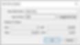
Step 2: An 'Edit bins' dialogue box would open which shows the range of values of the Sales field. It also suggests the size of bin which you can change as per your requirement. I am setting the size of bins as 500. Click on 'OK'.
Step 3: If you will observe the Data pane now. You will see a new field in the dimensions section named as 'Sales (bin)'. Drag this field into the column shelf as shown below. You will have your histogram.


The visualization is more concise now and hence the objective was reached.
Box plot
A boxplot is a graph that gives you a good indication of how the values in the data are spread out.
It displays the distribution of data using 5 indicators : minimum, first quartile (Q1), median, third quartile (Q3) and maximum.
It also tells you if your data is symmetrical, how your data is grouped or skewed.
We will discuss two ways of building a boxplot. We will make a boxplot showing the Discount per Region for each Segment.
Method 1:
This method is pretty straightforward.
First drag 'Segment' field and then the 'Region' field from data pane to the columns shelf.
From the ' 'Discount' field to the rows shelf.
From the 'Show Me' tab select the boxplot option. This will change the settings we made in the previous step but don't worry.
Now drag the 'Region' field from the marks card to the column shelf after the 'Segment' field and change the 'Discount' field to dimension from the dropdown menu in the row shelf.
Drag the 'Segment' field from the data pane to and drop it on the 'Color' option on the marks card.
You will get the following boxplot.

Method 2:
Step 1: First drag 'Segment' field and then the 'Region' field from data pane to the columns shelf.
Step 2: From the ' 'Discount' field to the rows shelf.
Step 3: Change the 'Discount' field to dimension from the dropdown menu in the row shelf. At this point you have a Gantt chart.
Step 4: Drag the 'Segment' field from the data pane to and drop it on the 'Color' option on the marks card.
Step 5: Now right click on the discount axis in the View area and select the 'Add reference line' option as shown below.

Step 6: In the dialogue box that opens select the boxplot option and click okay. You can also explore the other option here.

You will get the following boxplot.

You should try to explore Tableau yourself, just play around with it and let your creativity shine, you will learn much more that way. Also, Keep an eye out for the next blog.
You maybe interested to check out the following blogs:
If you need implementation for any of the topics mentioned above or assignment help on any of its variants, feel free to contact us.
