Nov 2, 2021

Bike Sharing Dataset - Regression

Updated: Nov 3, 2021

Description :

This dataset contains the hourly and daily count of rental bikes between the years 2011 and 2012 in the Capital bike share system with the corresponding weather and seasonal information.

Bike sharing systems are new generation of traditional bike rentals where whole process from membership, rental and return back has become automatic. Through these systems, user is able to easily rent a bike from a particular position and return back at another position. Currently, there are about over 500 bike-sharing programs around the world which is composed of over 500 thousands bicycles. Today, there exists great interest in these systems due to their important role in traffic, environmental and health issues.

Apart from interesting real world applications of bike sharing systems, the characteristics of data being generated by these systems make them attractive for the research. Opposed to other transport services such as bus or subway, the duration of travel, departure and arrival position is explicitly recorded in these systems. This feature turns bike sharing system into a virtual sensor network that can be used for sensing mobility in the city. Hence, it is expected that most of important events in the city could be detected via monitoring these data.

Recommended Model :

Algorithms to be used: Regression, SVM, RandomForestRegressor etc.

Recommended Project :

Demand forecast for Bike sharing

Dataset link:

https://www.kaggle.com/uciml/sms-spam-collection-dataset

Overview of data

Detailed overview of dataset:

- Rows = 731

- Columns= 17

Both hour.csv and day.csv have the following fields, except hr which is not available in day.csv

instant: record index
dteday : date
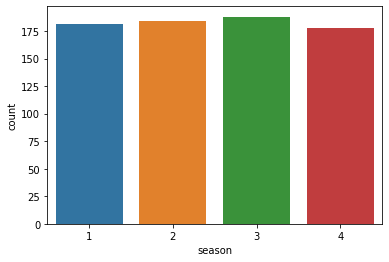
season : season (1:springer, 2:summer, 3:fall, 4:winter)
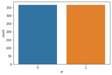
yr : year (0: 2011, 1:2012)
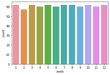
mnth : month ( 1 to 12)
hr : hour (0 to 23)
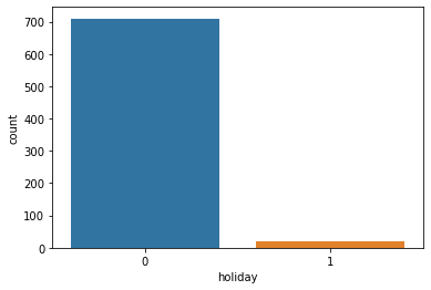
holiday : weather day is holiday or not (extracted from [Web Link])
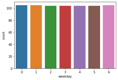
weekday : day of the week
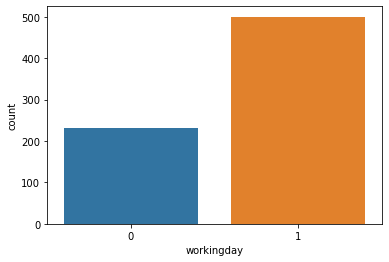
workingday : if day is neither weekend nor holiday is 1, otherwise is 0.
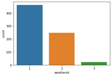
weathersit :

1: Clear, Few clouds, Partly cloudy, Partly cloudy
2: Mist + Cloudy, Mist + Broken clouds, Mist + Few clouds, Mist
3: Light Snow, Light Rain + Thunderstorm + Scattered clouds, Light Rain + Scattered clouds
4: Heavy Rain + Ice Pallets + Thunderstorm + Mist, Snow + Fog

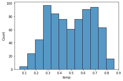
11. temp : Normalized temperature in Celsius. The values are derived via

(t-tmin)/(tmax-tmin), tmin=-8, t_max=+39 (only in hourly scale)

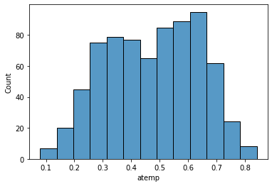
12. atemp: Normalized feeling temperature in Celsius. The values are derived via

(t-tmin)/(tmax-tmin), tmin=-16, t_max=+50 (only in hourly scale)

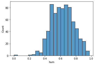
13. hum: Normalized humidity. The values are divided to 100 (max)

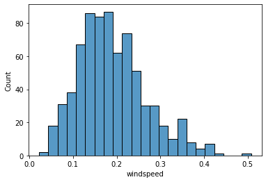
14. windspeed: Normalized wind speed. The values are divided to 67 (max)

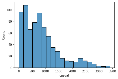
15. casual: count of casual users

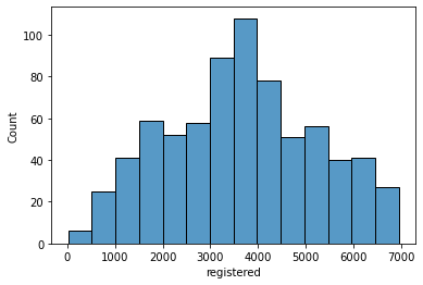
16. registered: count of registered users

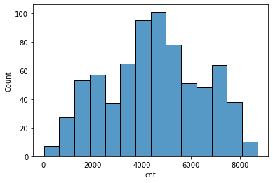
17. cnt: count of total rental bikes including both casual and registered

for further more information please go through the following link, http://archive.ics.uci.edu/ml/datasets/Bike+Sharing+Dataset

EDA [CODE]

import pandas as pd  
# load data data = pd.read_csv('spam.csv') 
data.head()

# check details of the dataframe 
data.info()

# check the no.of missing values in each column 
data.isna().sum()

# statistical information about the dataset 
data.describe()

# data distribution  

import seaborn as sns 
import matplotlib.pyplot as plt

sns.countplot(x='season', data=data) 
plt.show()

sns.countplot(x='yr', data=data) 
plt.show()

sns.countplot(x='mnth', data=data) 
plt.show()

sns.countplot(x='holiday', data=data) 
plt.show()

sns.countplot(x='weekday', data=data) 
plt.show()

sns.countplot(x='workingday', data=data) 
plt.show()

sns.countplot(x='weathersit', data=data) 
plt.show()


sns.histplot(data['hum'],  kde=False)
plt.show()

sns.histplot(data['temp'], kde= False)
plt.show()

sns.histplot(data['atemp'], kde=False)
plt.show()

sns.histplot(data['windspeed'], kde=False)
plt.show()

sns.histplot(data['casual'], kde=False)
plt.show()

sns.histplot(data['registered'], kde=False)
plt.show()

sns.histplot(data['cnt'], kde=False)
plt.show()