Skin Disease Classification Using Deep Learning: Part 1
- Sep 3, 2024
- 7 min read
Skin disease classification using images is a critical application in the field of medical diagnostics. Accurate classification of skin conditions can significantly aid dermatologists in early diagnosis and treatment planning. In this blog, we'll walk you through the process of building a skin disease classification model using deep learning. This tutorial is designed to be beginner-friendly, offering explanations at each step to ensure a solid understanding of the process. By the end, you'll have a functional model that can classify images of skin diseases into different categories.
Dataset
The dataset used in this project is the HAM10000 dataset, which consists of 10,015 images of different skin lesions, classified into seven categories: melanocytic nevi (nv), melanoma (mel), benign keratosis-like lesions (bkl), basal cell carcinoma (bcc), actinic keratoses (akiec), vascular lesions (vasc), and dermatofibroma (df). This dataset is commonly used for research in skin disease classification and provides a good variety of images for training robust models.
Step-by-Step Explanation of the Code
1. Import Necessary Libraries
First, we import the necessary libraries that will be used throughout the project. This includes libraries for data manipulation, machine learning, and image processing.
from numpy.random import seed
seed(101)
from tensorflow import set_random_seed
set_random_seed(101)

import pandas as pd
import numpy as np

import tensorflow
from tensorflow.keras.layers import Dense, Dropout
from tensorflow.keras.optimizers import Adam
from tensorflow.keras.metrics import categorical_crossentropy
from tensorflow.keras.preprocessing.image import ImageDataGenerator
from tensorflow.keras.models import Model
from tensorflow.keras.callbacks import EarlyStopping, ReduceLROnPlateau, ModelCheckpoint

import os

from sklearn.metrics import confusion_matrix
from sklearn.model_selection import train_test_split
import itertools
import shutil
import matplotlib.pyplot as plt
# %matplotlib inline
2. Directory Setup
We begin by setting up the directory structure to organize the dataset into training and validation folders. This structure is essential for the ImageDataGenerator to work correctly.
os.listdir('../input')

base_dir = 'base_dir'
os.mkdir(base_dir)

train_dir = os.path.join(base_dir, 'train_dir')
os.mkdir(train_dir)

val_dir = os.path.join(base_dir, 'val_dir')
os.mkdir(val_dir)
Output :
Next, we create subdirectories for each class within the training and validation directories.
nv = os.path.join(train_dir, 'nv')
os.mkdir(nv)
mel = os.path.join(train_dir, 'mel')
os.mkdir(mel)
bkl = os.path.join(train_dir, 'bkl')
os.mkdir(bkl)
bcc = os.path.join(train_dir, 'bcc')
os.mkdir(bcc)
akiec = os.path.join(train_dir, 'akiec')
os.mkdir(akiec)
vasc = os.path.join(train_dir, 'vasc')
os.mkdir(vasc)
df = os.path.join(train_dir, 'df')
os.mkdir(df)

nv = os.path.join(val_dir, 'nv')
os.mkdir(nv)
mel = os.path.join(val_dir, 'mel')
os.mkdir(mel)
bkl = os.path.join(val_dir, 'bkl')
os.mkdir(bkl)
bcc = os.path.join(val_dir, 'bcc')
os.mkdir(bcc)
akiec = os.path.join(val_dir, 'akiec')
os.mkdir(akiec)
vasc = os.path.join(val_dir, 'vasc')
os.mkdir(vasc)
df = os.path.join(val_dir, 'df')
os.mkdir(df)
3. Load and Prepare the Dataset
We load the metadata file associated with the HAM10000 dataset, which contains information about each image, including the type of lesion.
df_data = pd.read_csv('../input/HAM10000_metadata.csv')

df_data.head()
Output :
4. Create Stratified Validation Set
To ensure that our training and validation sets are representative of the overall dataset, we create a stratified validation set. This process involves identifying and separating duplicate lesion IDs to avoid data leakage.
df = df_data.groupby('lesion_id').count()
df = df[df['image_id'] == 1]
df.reset_index(inplace=True)

def identify_duplicates(x):
    unique_list = list(df['lesion_id'])
    if x in unique_list:
        return 'no_duplicates'
    else:
        return 'has_duplicates'

df_data['duplicates'] = df_data['lesion_id']
df_data['duplicates'] = df_data['duplicates'].apply(identify_duplicates)

df = df_data[df_data['duplicates'] == 'no_duplicates']

y = df['dx']
_, df_val = train_test_split(df, test_size=0.17, random_state=101, stratify=y)
Output
Create a train set that excludes images that are in the val set
In this section we Excludes the those images which are available in validation Set
def identify_val_rows(x):
    val_list = list(df_val['image_id'])

    if str(x) in val_list:
        return 'val'
    else:
        return 'train'


df_data['train_or_val'] = df_data['image_id']
df_data['train_or_val'] = df_data['train_or_val'].apply(identify_val_rows)

df_train = df_data[df_data['train_or_val'] == 'train']

print(len(df_train))
print(len(df_val))

df_train['dx'].value_counts()

df_val['dx'].value_counts()
Output :
5. Transfer Images to Folders
We now transfer the images into the appropriate folders for training and validation. This step ensures that our model will be able to access the images correctly during training.
df_data.set_index('image_id', inplace=True)

folder_1 = os.listdir('../input/ham10000_images_part_1')
folder_2 = os.listdir('../input/ham10000_images_part_2')

train_list = list(df_train['image_id'])
val_list = list(df_val['image_id'])

for image in train_list:
    fname = image + '.jpg'
    label = df_data.loc[image,'dx']
    if fname in folder_1:
        src = os.path.join('../input/ham10000_images_part_1', fname)
        dst = os.path.join(train_dir, label, fname)
        shutil.copyfile(src, dst)
    if fname in folder_2:
        src = os.path.join('../input/ham10000_images_part_2', fname)
        dst = os.path.join(train_dir, label, fname)
        shutil.copyfile(src, dst)

for image in val_list:
    fname = image + '.jpg'
    label = df_data.loc[image,'dx']
    if fname in folder_1:
        src = os.path.join('../input/ham10000_images_part_1', fname)
        dst = os.path.join(val_dir, label, fname)
        shutil.copyfile(src, dst)
    if fname in folder_2:
        src = os.path.join('../input/ham10000_images_part_2', fname)
        dst = os.path.join(val_dir, label, fname)
        shutil.copyfile(src, dst)
Display result:
print(len(os.listdir('base_dir/train_dir/nv')))
print(len(os.listdir('base_dir/train_dir/mel')))
print(len(os.listdir('base_dir/train_dir/bkl')))
print(len(os.listdir('base_dir/train_dir/bcc')))
print(len(os.listdir('base_dir/train_dir/akiec')))
print(len(os.listdir('base_dir/train_dir/vasc')))
print(len(os.listdir('base_dir/train_dir/df')))

print(len(os.listdir('base_dir/val_dir/nv')))
print(len(os.listdir('base_dir/val_dir/mel')))
print(len(os.listdir('base_dir/val_dir/bkl')))
print(len(os.listdir('base_dir/val_dir/bcc')))
print(len(os.listdir('base_dir/val_dir/akiec')))
print(len(os.listdir('base_dir/val_dir/vasc')))
print(len(os.listdir('base_dir/val_dir/df')))
Output :
6. Augment the Training Data
Data augmentation is crucial for improving the generalization of our model. We use the ImageDataGenerator to generate additional images by applying transformations like rotation, zooming, and flipping.
class_list = ['mel','bkl','bcc','akiec','vasc','df']

for item in class_list:
    aug_dir = 'aug_dir'
    os.mkdir(aug_dir)
    img_dir = os.path.join(aug_dir, 'img_dir')
    os.mkdir(img_dir)

    img_class = item
    img_list = os.listdir('base_dir/train_dir/' + img_class)

    for fname in img_list:
        src = os.path.join('base_dir/train_dir/' + img_class, fname)
        dst = os.path.join(img_dir, fname)
        shutil.copyfile(src, dst)

    path = aug_dir
    save_path = 'base_dir/train_dir/' + img_class

    datagen = ImageDataGenerator(
        rotation_range=180,
        width_shift_range=0.1,
        height_shift_range=0.1,
        zoom_range=0.1,
        horizontal_flip=True,
        vertical_flip=True,
        fill_mode='nearest')

    batch_size = 50
    aug_datagen = datagen.flow_from_directory(path,
                                               save_to_dir=save_path,
                                               save_format='jpg',
                                               target_size=(224,224),
                                               batch_size=batch_size)

    num_aug_images_wanted = 6000
    num_files = len(os.listdir(img_dir))
    num_batches = int(np.ceil((num_aug_images_wanted-num_files)/batch_size))

    for i in range(0,num_batches):
        imgs, labels = next(aug_datagen)

    shutil.rmtree('aug_dir')
Output :
print(len(os.listdir('base_dir/train_dir/nv')))
print(len(os.listdir('base_dir/train_dir/mel')))
print(len(os.listdir('base_dir/train_dir/bkl')))
print(len(os.listdir('base_dir/train_dir/bcc')))
print(len(os.listdir('base_dir/train_dir/akiec')))
print(len(os.listdir('base_dir/train_dir/vasc')))
print(len(os.listdir('base_dir/train_dir/df')))
Output :
print(len(os.listdir('base_dir/val_dir/nv')))
print(len(os.listdir('base_dir/val_dir/mel')))
print(len(os.listdir('base_dir/val_dir/bkl')))
print(len(os.listdir('base_dir/val_dir/bcc')))
print(len(os.listdir('base_dir/val_dir/akiec')))
print(len(os.listdir('base_dir/val_dir/vasc')))
print(len(os.listdir('base_dir/val_dir/df')))
Output :
Visualize 50 Augmented Images
def plots(ims, figsize=(12,6), rows=5, interp=False, titles=None): # 12,6
    if type(ims[0]) is np.ndarray:
        ims = np.array(ims).astype(np.uint8)
        if (ims.shape[-1] != 3):
            ims = ims.transpose((0,2,3,1))
    f = plt.figure(figsize=figsize)
    cols = len(ims)//rows if len(ims) % 2 == 0 else len(ims)//rows + 1
    for i in range(len(ims)):
        sp = f.add_subplot(rows, cols, i+1)
        sp.axis('Off')
        if titles is not None:
            sp.set_title(titles[i], fontsize=16)
        plt.imshow(ims[i], interpolation=None if interp else 'none')

plots(imgs, titles=None)
Output :
7. Set Up the Generators
Now, we set up the image generators for training and validation using the ImageDataGenerator with preprocessing applied.
train_path = 'base_dir/train_dir'
valid_path = 'base_dir/val_dir'

num_train_samples = len(df_train)
num_val_samples = len(df_val)
train_batch_size = 10
val_batch_size = 10
image_size = 224

train_steps = np.ceil(num_train_samples / train_batch_size)
val_steps = np.ceil(num_val_samples / val_batch_size)

datagen = ImageDataGenerator(preprocessing_function= \
    tensorflow.keras.applications.mobilenet.preprocess_input)

train_batches = datagen.flow_from_directory(train_path,
                                            target_size=(image_size,image_size),
                                            batch_size=train_batch_size)

valid_batches = datagen.flow_from_directory(valid_path,
                                            target_size=(image_size,image_size),
                                            batch_size=val_batch_size)

test_batches = datagen.flow_from_directory(valid_path,
                                            target_size=(image_size,image_size),
                                            batch_size=1,
                                            shuffle=False)
Output :
8. Build and Train the CNN Model
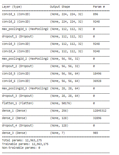
We then build a convolutional neural network (CNN) model using Keras. The model architecture consists of several convolutional layers followed by max-pooling layers and dropout for regularization. Finally, we compile and train the model using the Adam optimizer and categorical cross-entropy loss.
from keras.layers import Flatten,Dense,Dropout,BatchNormalization,Conv2D, MaxPool2D
from keras.optimizers import Adam
from keras.callbacks import ReduceLROnPlateau
from keras.preprocessing.image import ImageDataGenerator

import matplotlib.pyplot as plt
from PIL import Image
import seaborn as sns
import numpy as np
import pandas as pd
import os
from tensorflow.keras.utils import to_categorical
from glob import glob

from keras.models import Sequential
import keras.models

input_shape = (224,224, 3)
num_classes = 7

model = Sequential()
model.add(Conv2D(32, kernel_size=(3, 3),activation='relu',padding = 'Same',input_shape=input_shape))
model.add(Conv2D(32,kernel_size=(3, 3), activation='relu',padding = 'Same',))
model.add(MaxPool2D(pool_size = (2, 2)))
model.add(Dropout(0.16))

model.add(Conv2D(32, kernel_size=(3, 3),activation='relu',padding = 'Same'))
model.add(Conv2D(32,kernel_size=(3, 3), activation='relu',padding = 'Same',))
model.add(MaxPool2D(pool_size = (2, 2)))
model.add(Dropout(0.20))

model.add(Conv2D(64, (3, 3), activation='relu',padding = 'same'))
model.add(Conv2D(64, (3, 3), activation='relu',padding = 'Same'))
model.add(MaxPool2D(pool_size=(2, 2)))
model.add(Dropout(0.25))

model.add(Flatten())
model.add(Dense(256, activation='relu'))
model.add(Dense(128, activation='relu'))
model.add(Dropout(0.4))
model.add(Dense(num_classes, activation='softmax'))
model.summary()

optimizer = Adam(lr=0.0001, beta_1=0.9, beta_2=0.999, epsilon=None, decay=0.0, amsgrad=False)

model.compile(optimizer = optimizer , loss = "categorical_crossentropy", metrics=["accuracy"])
Output :
We also define a learning rate reduction callback to adjust the learning rate during training if the validation accuracy plateaus.
learning_rate_reduction = ReduceLROnPlateau(monitor='val_acc',
                                            patience=4,
                                            verbose=1,
                                            factor=0.5,
                                            min_lr=0.00001)

epochs = 30
batch_size = 10
history = model.fit_generator(train_batches, steps_per_epoch=train_steps,
                    validation_data=valid_batches,
                    validation_steps=val_steps,
                    epochs=epochs, verbose=1,
                    callbacks=[learning_rate_reduction])
Output :
9. Evaluate the Model
After training, we evaluate the model's performance on the validation set using various metrics such as loss, accuracy, and top-k categorical accuracy.
val_loss, val_cat_acc = \
model.evaluate_generator(test_batches,
                        steps=len(df_val))

print('val_loss:', val_loss)
print('val_cat_acc:', val_cat_acc)

model.save("model.h5")
Output :
10. Visualize the Training Process
We can visualize the training process by plotting the training and validation loss and accuracy over the epochs.
import matplotlib.pyplot as plt

acc = history.history['acc']
val_acc = history.history['val_acc']
loss = history.history['loss']
val_loss = history.history['val_loss']
epochs = range(1, len(acc) + 1)

plt.plot(epochs, loss, 'bo', label='Training loss')
plt.plot(epochs, val_loss, 'b', label='Validation loss')
plt.title('Training and validation loss')
plt.legend()
plt.figure()

plt.plot(epochs, acc, 'bo', label='Training cat acc')
plt.plot(epochs, val_acc, 'b', label='Validation cat acc')
plt.title('Training and validation cat accuracy')
plt.legend()
plt.figure()

plt.show()
Output :
11. Confusion Matrix and Classification Report
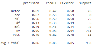
Finally, we generate a confusion matrix and a classification report to better understand the model's performance across different classes.
from sklearn.metrics import classification_report, confusion_matrix

predictions = model.predict_generator(test_batches, steps=len(df_val), verbose=1)

cm = confusion_matrix(test_batches.classes, predictions.argmax(axis=1))

cm_plot_labels = ['akiec', 'bcc', 'bkl', 'df', 'mel','nv', 'vasc']

def plot_confusion_matrix(cm, classes,
                          normalize=False,
                          title='Confusion matrix',
                          cmap=plt.cm.Blues):
    if normalize:
        cm = cm.astype('float') / cm.sum(axis=1)[:, np.newaxis]
        print("Normalized confusion matrix")
    else:
        print('Confusion matrix, without normalization')
    print(cm)

    plt.imshow(cm, interpolation='nearest', cmap=cmap)
    plt.title(title)
    plt.colorbar()
    tick_marks = np.arange(len(classes))
    plt.xticks(tick_marks, classes, rotation=45)
    plt.yticks(tick_marks, classes)

    fmt = '.2f' if normalize else 'd'
    thresh = cm.max() / 2.
    for i, j in itertools.product(range(cm.shape[0]), range(cm.shape[1])):
        plt.text(j, i, format(cm[i, j], fmt),
                 horizontalalignment="center",
                 color="white" if cm[i, j] > thresh else "black")

    plt.ylabel('True label')
    plt.xlabel('Predicted label')
    plt.tight_layout()

plot_confusion_matrix(cm, cm_plot_labels, title='Confusion Matrix')

y_pred = np.argmax(predictions, axis=1)
y_true = test_batches.classes

report = classification_report(y_true, y_pred, target_names=cm_plot_labels)

print(report)
Output :
In this blog, we walked through the step-by-step process of building a skin disease classification model using a convolutional neural network (CNN). We started with data preparation, moved on to model training, and finally evaluated the model's performance. This process demonstrates the power of deep learning in medical imaging and how it can be applied to real-world problems like skin disease classification. By following these steps, you can create your own skin disease classification model and further experiment with different architectures and techniques to improve its accuracy. in the second part we will see how to use pre-trained convolutional neural network (CNN) architecture for image classification tasks.
If you require any assistance with this project or Machine Learning projects, please do not hesitate to contact us. We have a team of experienced developers who specialize in Machine Learning and can provide you with the necessary support and expertise to ensure the success of your project. You can reach us through our website or by contacting us directly via email or phone.


Comments