Image Classification Using Machine Learning Techniques
- Aug 17, 2020
- 5 min read
Updated: Mar 25, 2021
Introduction:
Image classification can be accomplished by any machine learning algorithms( logistic regression, random forest, and SVM). But all the machine learning algorithms required proper features for doing the classification. If you feed the raw image into the classifier, it will fail to classify the images properly and the accuracy of the classifier would be less.
CNN ( convolution neural network ) extracts the features from the images and it handles the entire feature engineering part. In normal CNN architecture, beginning layers are extracting the low-level features and end level layers extract high-level features from the image.
Before CNN, we need to spend time selecting the proper features for classifying the image. There are so many handcrafted features available( local feature, global feature), but it will take so much time to select the proper features for a solution( image classification) and selecting the proper classification model. CNN handles all these problems and the accuracy of CNN is higher compared with the normal classifier.
Different CNN Architectures are listed below
LetNet
AlexNet
VGG16
VGG19
Google Inception
Resnet.
In this Blog, a simple CNN model and VGG-16(Transfer Learning) Model is discussed.
1. Simple CNN Architechture:

Fig-1: CNN Architecture
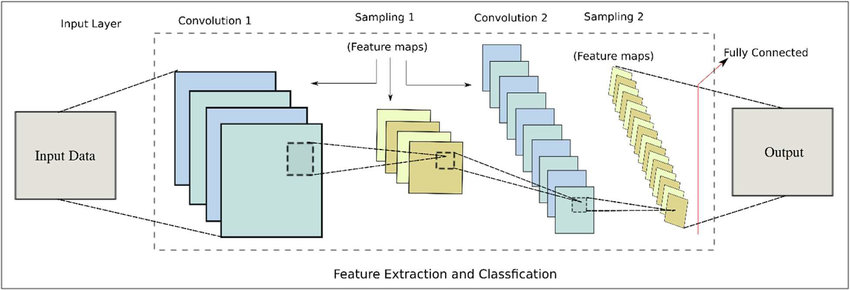
Fig-2: Simple CNN Architecture(With more labels)
CNN Architecture steps:
Let the image size is 100X100, and stride=1, with ongoing 1st convolution with 200 filters and then 2nd convolution with 100 filters
Input Layer: The input images are loaded to this layer & the produced output is used to feed the convolution layers. Several image processing techniques such as resizing of the image to 40x40 pixels from 50X50 are applied. In our case, the dataset consists of the image and parameters are defining the image dimensions (100X100 pixels) and the number of channels is 3 for RGB.
Convolutional Layer: In this layer, the convolution between input images with a set of learnable features or filters is carried out. By finding rough feature matches, in the same position for two images, CNN gets a lot better at seeing the similarity than whole image matching schemes. There are two convolution layers in our model with the receptive fields or kernel size of 3X3, the stride is set to 1. The first convolution layer learns 200 filters and the second one learns 100 filters.
ReLU Layer: This layer removes the negative values from the filtered images and replaces them with zeros. For a given input value y, the ReLU layer computes output f(y) as y if y>0, else 0, or simply the activation is the threshold at zero. The first layer is the Conv2D layer with 200 filters and the filter size or the kernel size of 3X3. In this first step, the activation function used is the ‘ReLu’. This ReLu function stands for the Rectified Linear Unit which will output the input directly if is positive, otherwise, it will output zero. The input size is also initialized as 100X100X3 for all the images to be trained and tested using this model
Pooling Layer: In this layer, the image stack is shrunk into a smaller size. The chosen window size is 2X2 with a stride of 1. For moving each window across the image, the maximum value is taken.
Convolutional Layer: The next layer is again a Conv2D layer with another 100 filters of the same filter size 3X3 and the activation function used is the ‘ReLu’. This Conv2D layer is followed by a MaxPooling2D layer with pool size 2X2.
Flatten(): In the next step, we use the Flatten() layer to flatten all the layers into a single 1D layer
Fully Connected Layer(FCN): This is the final layer where the actual classification happens. All filtered & shrunk images are stacked up. It passes the flattened output to the output layer where the SoftMax classifier is used to predict the labels.
At last, The dropout layers are added after the convolution & pooling layers to overcome the problem of overfitting to some extent. In our case it 0.5. This layer arbitrarily turns off a fraction of neurons during the training process, which reduces the habituation on the training set by some amount. The fraction of neurons to turn off is decided by a hyperparameter, which can be tuned accordingly. The loss function used here is categorical cross-entropy and the Keras optimizer used is Adam. Data Augmentation methods are also applied for image data such as horizontal & vertical flip, range of rotation, width and height shift, etc. It is required to obtain more data for training in general and adds it to the training set, also used to reduce overfitting.
The process diagram is shown below

2. VGG-16(Transfer Learning):

Fig-3: VGG-16 Architecture
VGG-16 model is used in case of the limited size of datasets, VGG-16 is a pretrained model used in transfer learning techniques, for this reason, we have to ignore the training the layers which are already trained.
The working process of VGG-16 has shown below

Working:
Due to the limited size dataset, it is difficult for learning algorithms to learn better features. As deep learning-based methods often require larger datasets, transfer learning is proposed to transfer learned knowledge from a source task to a related target task. Transfer learning has helped with learning in a significant way as long as it has a close relationship.
First, we import the necessary libraries then we labeled the images as 0 and 1, in case of multiclass-classification we can use more. Pre-processing steps include resizing to 224×224 pixels, conversion to array format, and scaling the pixel intensities in the input image to the range [-1, 1].
Here the input image shape is 224X224X3. And we trained it using MobileNetV2 with weights of ImageNet.(In transfer learning VGG-16 Model the image size should be resized into 224X224)
Then the MaxPooling layer is used with pool size 7X7.
In the next step, we use the Flatten() layer to flatten all the layers into a single 1D layer.
After the Flatten layer, we use the Dropout (0.5) layer to prevent the model from overfitting.
Finally, towards the end, we use the Dense layer with 128 units, and the activation function as ‘ReLu’.
The last layer of our model will be another Dense Layer, with only two units and the activation function used will be the ‘Softmax’ function. The softmax function outputs a vector which will represent the probability distributions of each of the input units. Here, two input units are used. The softmax function will output a vector with two probability distribution values.
After building the model, we compile the model and define the loss function and optimizer function. In this model, we use the ‘Adam’ Optimizer and the ‘Binary Cross Entropy’ as the Loss function for training purposes.
Finally, the VGG-16 model along with the cascade classifier is trained for 10 epochs with two classes. (In case of multi-class we have to train using multi-classes).
So In this manner, these are the two methods/Techniques explained above that can be used in Image classification.
Thank You!


Comments